Overfitting happens when a trading strategy captures quirks in historical data rather than a pattern that survives new conditions. Walk forward testing checks that weakness by repeatedly selecting parameters on earlier data, then evaluating them on a later period that did not influence the selection.
The distinction matters: a profitable backtest shows what worked in a historical simulation. A properly designed walk forward test asks whether your strategy development process could have produced useful decisions as time passed. Within trading strategy backtesting software, that requires more than an optimizer and an attractive equity curve.
How Trading Strategies Become Overfit
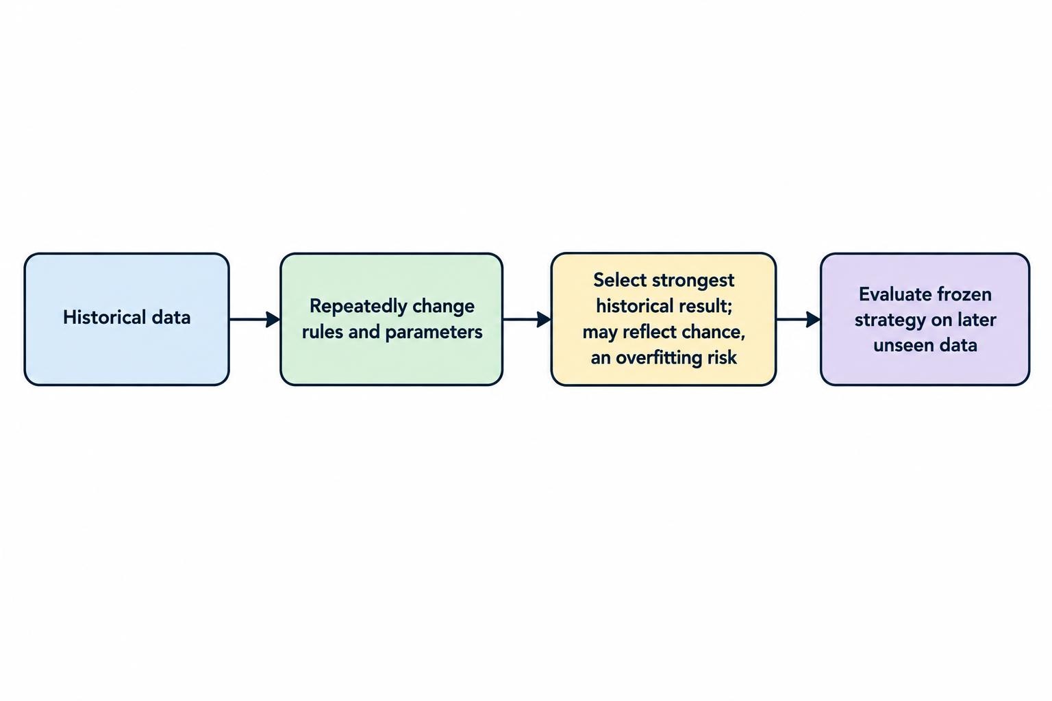
Overfitting does not require machine learning or hundreds of indicators. A simple strategy can become overfit when you repeatedly adjust its entry rules, stop distance, trading hours or instrument selection after inspecting the results. Every revision gives the historical sample another opportunity to influence the final design.
Suppose you test 12 lookback periods, 10 entry thresholds and five exit settings. That produces 600 parameter combinations. Choosing the strongest result does not establish that the winner has a repeatable edge. The selection process can favor a combination that benefited from chance. The research paper The Probability of Backtest Overfitting examines this problem and methods for assessing selection failure.
Count informal experiments too. Rejecting several markets, changing the start date and removing an awkward trading session are research decisions, even if your optimizer never records them. A short parameter list can hide a very long search.
One useful diagnostic is parameter sensitivity. Compare the selected settings with nearby alternatives. If a 40-period lookback performs reasonably but 39 and 41 collapse, investigate the isolated peak. A broad region of acceptable results is a better candidate for further testing, though it is not proof of future profitability.
What Walk Forward Testing Actually Tests
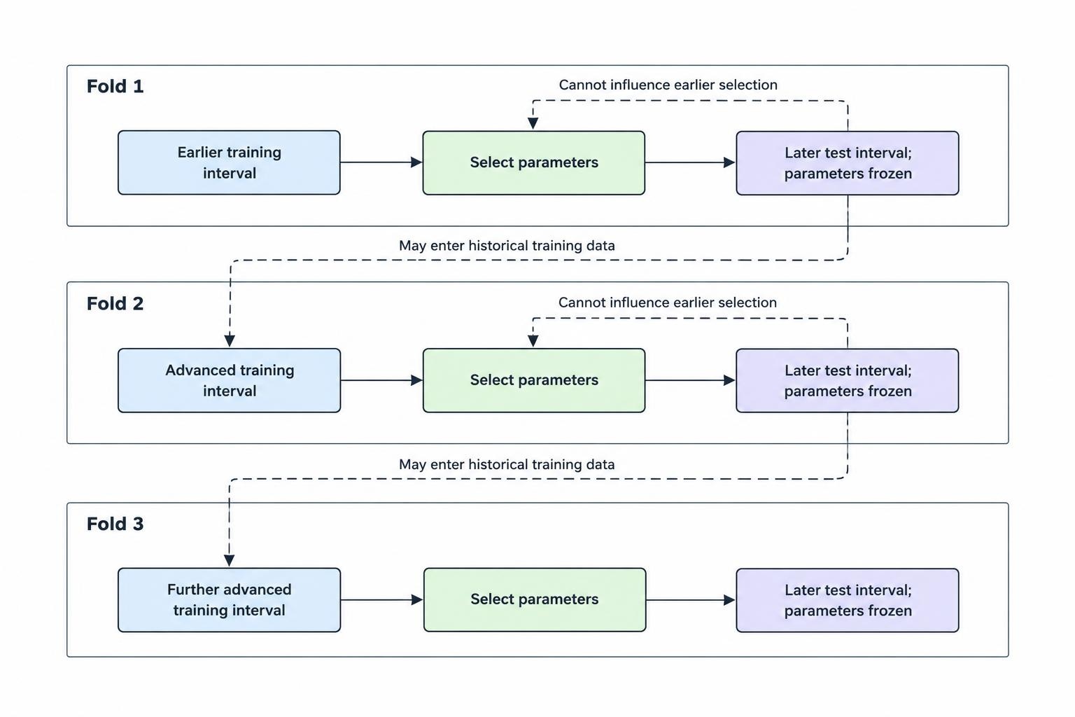
A walk forward test divides history into a sequence of training and subsequent test periods. Select parameters using the training period, freeze those choices for the next test period, then advance the dates and repeat. Walk forward optimization is the repeated calibration step; walk forward testing evaluates the resulting decisions outside their selection windows. QuantConnect’s walk forward optimization documentation demonstrates scheduled parameter adjustment using trailing data.
The object being tested is therefore a procedure, not one permanent parameter set. That procedure includes the strategy rules, parameter search, selection objective, training window and recalibration schedule. Changing any of these after inspecting test results creates another research version.
A Walk Forward Testing Example
Consider a hypothetical daily trend strategy. Its research protocol specifies three years of training data, three months of testing and quarterly parameter updates. The following schedule illustrates four consecutive folds, where a fold means one training and test pair.
| Fold | Training period | Test period |
|---|---|---|
| 1 | January 2020–December 2022 | January–March 2023 |
| 2 | April 2020–March 2023 | April–June 2023 |
| 3 | July 2020–June 2023 | July–September 2023 |
| 4 | October 2020–September 2023 | October–December 2023 |
At each cutoff, the optimizer uses only information available by that date. The selected configuration then trades the next quarter without retrospective adjustment. These dates illustrate the mechanics, not a recommended window length.
Earlier test data can legitimately enter a later training window. March 2023 is unseen when the first configuration is selected, but it is historical information by April. That is not leakage. Using April’s results to choose the configuration supposedly deployed in January would be.
Choose Rolling or Anchored Training Windows
A rolling window keeps a fixed training length and drops older observations as new ones arrive. An anchored window keeps the original start date and expands the training sample at each update. In the example above, anchored training would continue to start in January 2020.
Choose the design to match the proposed live process. Rolling training discards older evidence by design; anchored training retains it. Neither choice deserves preference simply because it produces a better historical chart.
Window length also needs to match the strategy’s information requirements. A strategy that holds positions for months needs a different evaluation horizon from one that trades throughout each session. Thousands of bars do not necessarily represent thousands of independent opportunities.
Before comparing window designs, check the inputs. Changing validation dates cannot repair revised economic releases, missing delisted securities or incorrect timestamps. The separate guide to historical data quality and backtesting bias covers those issues. Treat clean data as a prerequisite, not something walk forward testing supplies.
Build a Walk Forward Test You Can Audit
Lock the Research Rules Before Running the Test
Write down the candidate parameters, selection metric, risk constraints, update schedule and rejection criteria before evaluating the test periods. Specify tie breaking too. Otherwise, two nearly identical training results can become an invitation to choose whichever configuration looks better later.
A hypothetical selection rule might maximize return after costs, subject to a drawdown ceiling and a minimum number of completed trades. Those constraints need a reason tied to the strategy and intended use. There is no universal trade count or training-to-test ratio that makes a backtest trustworthy.
If you compare several model families or tune machine learning settings, keep that selection inside the training window, using an internal chronological validation split where appropriate. The next outer test period must remain outside that decision.
Fit Data Transformations Inside Each Training Window
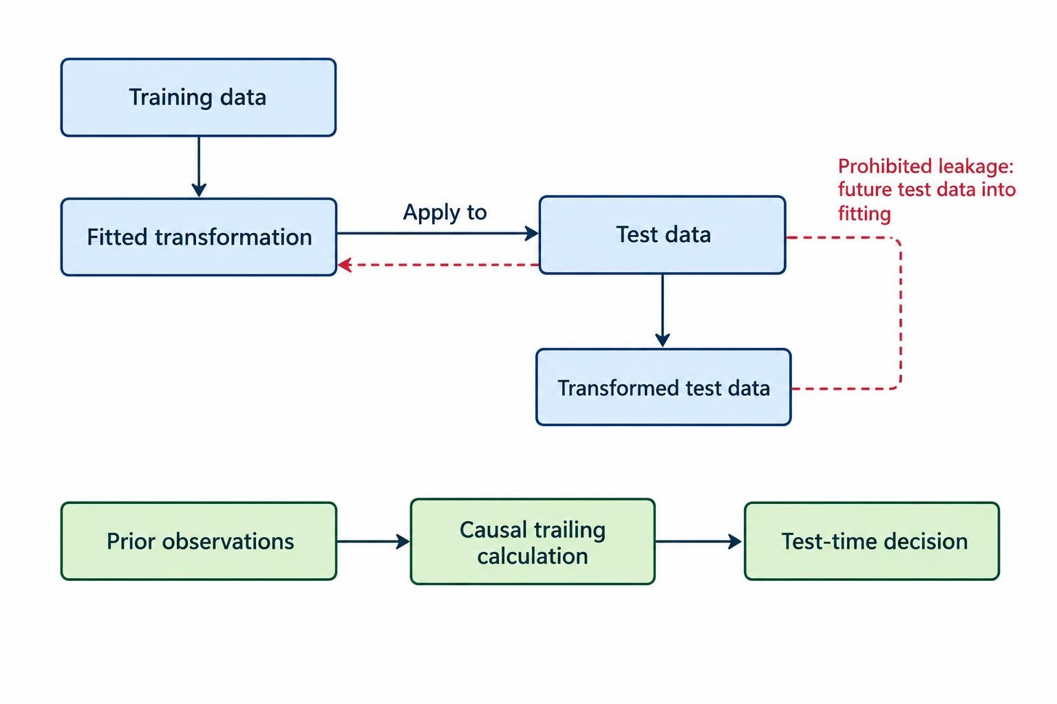
Leakage can enter before a trading signal is calculated. Scaling values using the full dataset, choosing features from all available history or filling missing observations using future information lets the test period influence model construction.
Fit learned transformations on the training data, then apply those fitted transformations to the test data. Repeat the fitting process at the next scheduled update. This separation applies to feature selection as well as preprocessing; scikit-learn’s data leakage guidance demonstrates how including test information can inflate evaluation results.
Distinguish learned transformations from ordinary causal calculations. A trailing moving average can use observations preceding the test period. It cannot use prices that had not arrived at the time of the simulated decision.
Check What Crosses the Training Boundary
For a chronological deployment test, do not randomly shuffle observations between training and testing. Preserve the direction of time. Where a separation is appropriate, scikit-learn’s TimeSeriesSplit documentation provides a gap setting that excludes observations from the end of each training split.
A gap is not an automatic cure. Consider a model trained to predict the next five trading days’ return. At the training cutoff, the latest observations may not yet have their full outcomes available. Exclude affected training examples until their outcomes would actually be known.
Choose exclusions from the information timeline, not an arbitrary percentage. Keep indicator warm-up separate: a strategy may need earlier prices to initialize its calculations, but warm-up activity should not contribute to reported test returns.
Model Costs and Position Changes at Every Update
Define commissions, spread, slippage and any relevant financing or borrow charges before comparing candidates. Apply a consistent execution model during parameter selection and testing. If training ignores costs but evaluation includes them, the optimizer is solving a different problem from the one you intend to trade.
Also decide what happens to open positions when parameters change. Do existing trades keep their original exit rules? Does the new configuration take control? Are positions closed and reopened? Each policy describes a different strategy.
Model the chosen transition and its costs explicitly. Do not restart every test window flat unless the proposed live process really does close positions at those boundaries. Otherwise, the simulation may discard inconvenient holdings and their losses.
Join Only the Test Returns
Build the headline equity curve from the consecutive test segments, excluding training performance. Preserve the capital, exposure and position treatment specified by the protocol.
For a simple hypothetical example, a $100,000 account gaining 5% in one test segment reaches $105,000. A subsequent 4% loss leaves $100,800. The combined return is 0.8%, not the 1% obtained by adding the percentages.
For a continuous account simulation, calculate portfolio statistics from the joined return series rather than averaging the Sharpe ratios or drawdowns reported for individual folds. Keep the fold reports as supporting records. Each fold needs its own record, the final chart is not enough.
Read the Results Beyond Net Profit
A positive combined return is a starting point for inspection. Check how that return was earned, how much risk supported it and whether the proposed recalibration process behaved consistently.
- Performance concentration: Identify whether one quarter, instrument or unusual event supplied most of the profit.
- Drawdown and recovery: Inspect losses across fold boundaries, not just inside each separately restarted report.
- Trading activity: Review turnover, exposure and completed trades alongside returns.
- Parameter movement: Investigate repeated jumps between distant settings, especially when training scores are nearly tied.
- Cost sensitivity: Recalculate results under predeclared, less favorable execution assumptions.
Compare the procedure with an appropriate simple benchmark and, where useful, a fixed-parameter version using consistent costs and exposure assumptions. This asks whether repeated optimization earns its extra complexity.
Do not interpret every weak test segment as proof of overfitting. Inspect data, execution assumptions and changes in trading conditions before drawing that verdict. Conversely, do not explain away every loss as a new market regime. A test needs permission to reject the strategy.
What the Software Should Record
When comparing algorithmic trading platforms, look beyond whether a product offers a walk forward button. You need control over date boundaries, training and testing lengths, parameter ranges, execution assumptions and position handling.
Require exportable results for every fold: selected parameters, training scores, test returns, trades and costs. Preserve the strategy version, dataset version, configuration and any random seed used by the search. Failed and rejected experiments belong in the research log too.
Check whether parallel jobs share model state or cached transformations. Separate test jobs should not inherit information learned from a later period. Faster optimization is useful only when the experiment remains valid; otherwise it produces misleading results at an impressive speed.
Keep a Final Test Outside the Development Loop
Walk forward testing can itself become overfit. If you repeatedly change the window length, scoring rule or strategy after reviewing the combined results, those results are now part of development. Calling them “out of sample” does not restore their independence.
Reserve a later holdout period where sufficient data exists. Finalize the full procedure before opening it, and do not use it to choose between competing versions. If the result prompts another redesign, treat that as a new development cycle rather than relabeling the same period as untouched evidence.
The next stage is paper trading the automated strategy with the same update schedule and risk rules. Use it to check operational behavior without treating simulated fills as proof of live execution quality.
Walk forward testing does not guarantee profitability. Its practical value is a stricter question: could the documented selection process have made these decisions using only what was available at the time? If the software cannot show that trail, the equity curve is not enough.